Introduction to Topological Data Analysis (TDA)

Hannah Schreiber & Vincent Rouvreau - Inria

Maintainer of the GUDHI library

Motivation

Data often have topological / geometric structure

How many mountains

How to identify:

• Small bump on the side of a bigger mountain?
• Independent mountains?

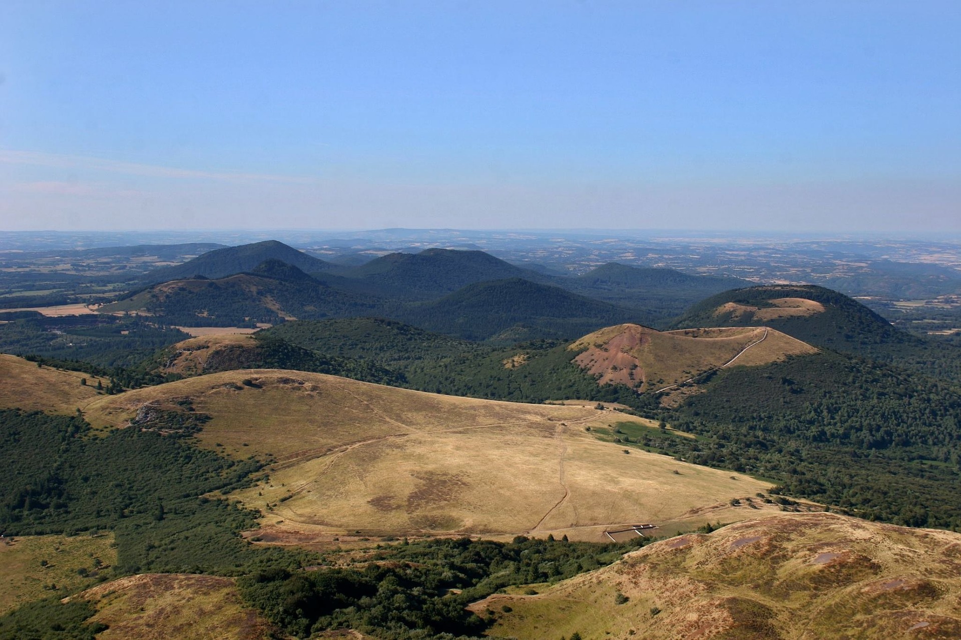
Prominence (topography) [source wikipedia]

Local maximum: how low do you need to go before you can reach a higher maximum?

Superlevelsets

Superlevelsets

Ok, but... In topology, we compute sublevelsets

From barcode to diagram

Interval (a, b) => Point (a,b)

Short bar => Point close to the diagonal

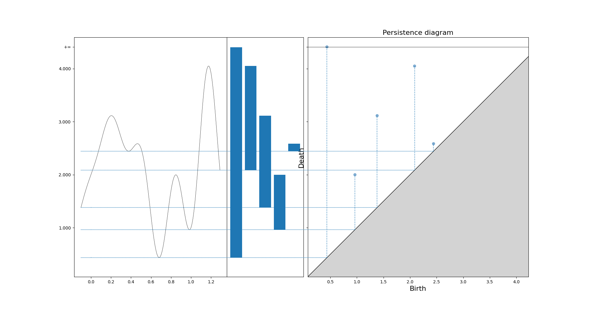
import matplotlib.pyplot as plt
import numpy as np
import gudhi as gd

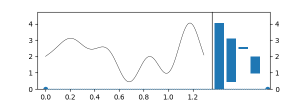
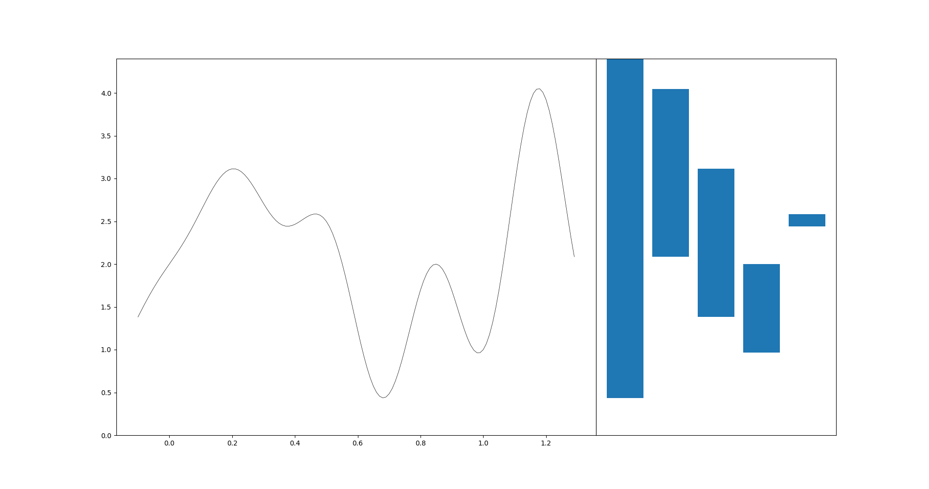
t = np.arange(-0.1, 1.3, 0.01)
s = np.sin(2 * np.pi * t) - t * np.cos(6 * np.pi * t) + 2

fig, axes = plt.subplots(ncols=2, sharey=True, figsize=(7, 1), gridspec_kw=dict(width_ratios=[4, 3], wspace=0))
fig.set_size_inches(9, 4)
axes[0].plot(t, s, "k", lw=0.5)

diag = gd.CubicalComplex(top_dimensional_cells=s).persistence()
_ = gd.plot_persistence_diagram(diag, legend=True, axes=axes[1])

Higher dimension

Loops are detected (cf. Puy Pariou)

Stability

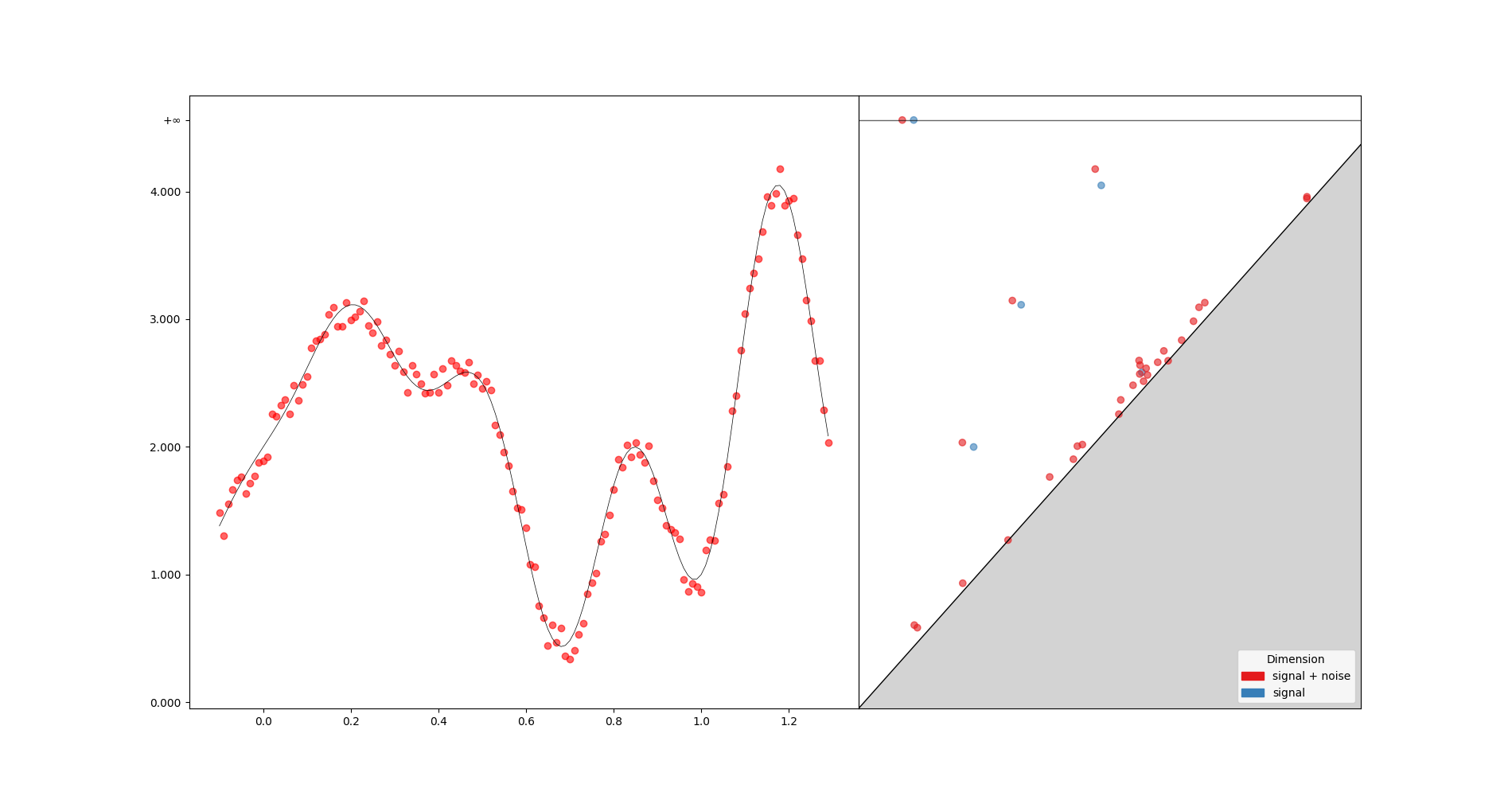
\begin{equation} \lVert f - g \rVert _\infty = sup _{x \in X} \left\{ \lvert f(x) - g(x) \rvert \right\} \end{equation}

Bottleneck distance: Partial matching, the rest matched with the diagonal. The worst pair defines the cost

Stability theorem: $$ d_B ( Dgm(f) - Dgm(g) ) \le \lVert f - g \rVert _\infty $$

Representations

Independent (?) problem: point clouds

Input: point set P

Assumption: P approaches some unknown ideal object

Sublevel sets on a point cloud

import matplotlib.pyplot as plt
import gudhi as gd
import numpy as np
import math

N=20
np.random.seed(0)
rand_angles = np.random.rand(N) * 2 * math.pi
X = np.stack((np.vectorize(math.cos)(rand_angles), np.vectorize(math.sin)(rand_angles)), axis=1)

fig, axes = plt.subplots(ncols=2, figsize=(4, 2)); fig.set_size_inches(12, 5)
axes[0].scatter(X[:,0],X[:,1], s=50)
axes[0].set_xlim(-2., 2.); axes[0].set_ylim(-2., 2.)

dgm = gd.AlphaComplex(points=X).create_simplex_tree().persistence()
gd.plot_persistence_barcode(dgm, legend=True, axes=axes[1])
plt.show()

ToMaTo

Introduction

${\rm ToMaTo}$ algorithm is exposed in the paper of Frédéric CHAZAL et al., Persistence-Based Clustering in Riemannian Manifolds [1], a clustering method based on the idea of topological persistence.

In short, the algorithm needs a density estimation (so to each point $x$ we associate a value $\hat{f}(x)$) and a neighborhood graph. First, it starts with a mode-seeking phase (naive hill-climbing) to build the initial clusters (each with its own mode), following the connected points in the neighborhood graph. Finally, it merges these initial clusters based on their prominence. This merging has a hierarchical nature, i.e. we always obtain the successive new clusters by merging two existing ones.

from sklearn import datasets
import matplotlib.pyplot as plt
import numpy as np

varied = datasets.make_blobs(n_samples=500, cluster_std=[1.0, 2.5, 0.5], random_state=170)[0]
x, y = varied.T
plt.scatter(x,y)
plt.show()

Construction

1. Graph

Default is KNN, can be a radius graph or set manually.

from gudhi.point_cloud.knn import KNearestNeighbors

nbrs = KNearestNeighbors(k=6)
indices = nbrs.fit_transform(varied)
for i in indices:
    Y = np.zeros((2,2))
    for j in range(len(i)):
        Y[0] = [varied[int(i[0])][0], varied[int(i[j])][0]]
        Y[1] = [varied[int(i[0])][1], varied[int(i[j])][1]]
        plt.plot(Y[0], Y[1], 'ro-')

plt.show()

2. Density

from sklearn.neighbors import KernelDensity

kde = KernelDensity(bandwidth=0.1).fit(varied)

z_kde = kde.score_samples(varied)
ax = plt.axes(projection='3d')
_ = ax.scatter(x, y, z_kde, c=z_kde)
plt.show()

from gudhi.clustering.tomato import Tomato

tomato = Tomato()
tomato.fit(varied)
tomato.plot_diagram()
plt.show()

tomato.n_clusters_=3
plt.scatter(x,y,c=tomato.labels_)
plt.show()

Benchmark [source]

%run ./scripts/plot_cluster_comparison.py

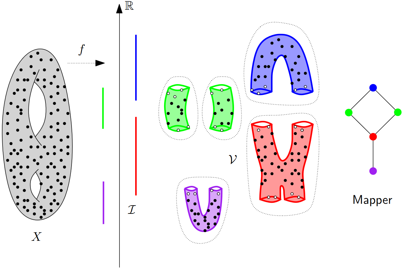
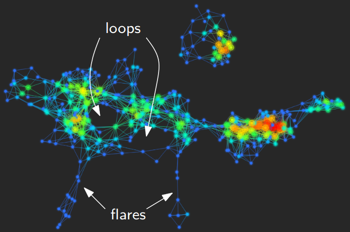
Mapper

Visualize topology on the data directly. Two types of applications:

• clustering
• feature selection

Principle: identify statistically relevant sub-populations through patterns (flares, loops)

Mapper in applications

3d shapes classification

Mapper in applications

breast cancer subtype identification

And so many other applications...

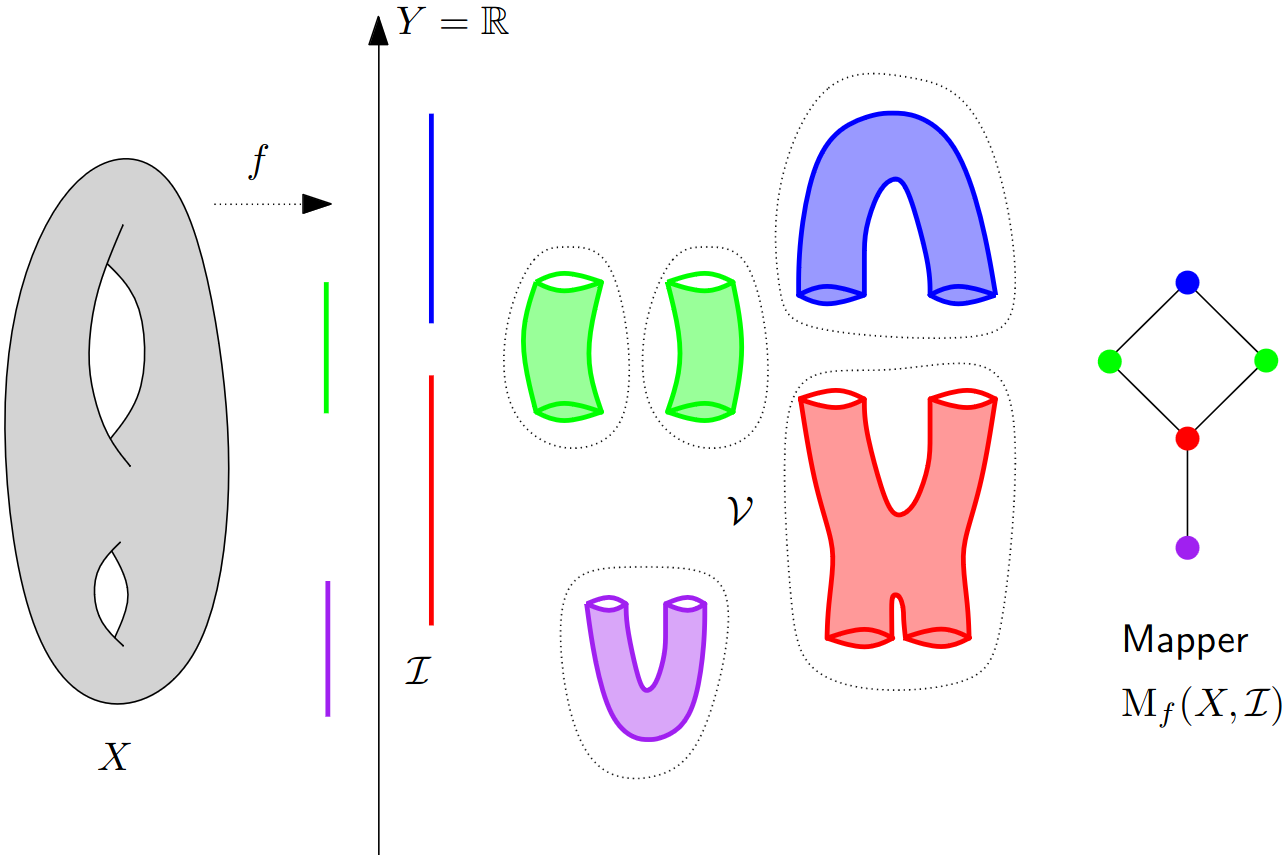
Mapper in the continuous setting

Mapper in practice